This post will be about using OmicsPLS to integrate two real datasets: transcriptomics and miRNA-omics from cancer patients These data are available freely on the JIVE website. They have been previously analyzed by JIVE (of course) with nice results, see the article associated with DOI:10.1214/12-AOAS597.
Downloading and reading the data
First, we load the packages that we will use. The zip file can be downloaded here. They contain the mRNA and miRNA files, probably after pre-processing by the authors (since the file names include “forInt”, meaning for integration..?). We read in the files, and center the columns around zero. For some reason, there are no gene IDs provided.
library(parallel)
library(tidyverse)
## ── Attaching packages ─────────────────────────────────────── tidyverse 1.3.0 ──
## ✓ ggplot2 3.3.3     ✓ purrr   0.3.4
## ✓ tibble  3.1.0     ✓ dplyr   1.0.4
## ✓ tidyr   1.1.2     ✓ stringr 1.4.0
## ✓ readr   1.4.0     ✓ forcats 0.5.1
## ── Conflicts ────────────────────────────────────────── tidyverse_conflicts() ──
## x dplyr::filter() masks stats::filter()
## x dplyr::lag()    masks stats::lag()
library(OmicsPLS)
##
## Attaching package: 'OmicsPLS'
## The following object is masked from 'package:stats':
##
##     loadings
# Files after unzipping
cat("List of files \n")
## List of files
list.files()
## [1] "FullExpforInt.txt"
## [2] "miRNAforInt.txt"
## [3] "Readme.txt"
## [4] "SubtypeLabels.txt"
# Read in files
miRNA = read_delim("miRNAforInt.txt",delim = ' ',
               escape_double = FALSE, col_names = FALSE, trim_ws = TRUE)
##
## ── Column specification ────────────────────────────────────────────────────────
## cols(
##   .default = col_double()
## )
## ℹ Use `spec()` for the full column specifications.
mRNA = read_delim("FullExpforInt.txt",delim = ' ',
               escape_double = FALSE, col_names = FALSE, trim_ws = TRUE)
##
## ── Column specification ────────────────────────────────────────────────────────
## cols(
##   .default = col_double()
## )
## ℹ Use `spec()` for the full column specifications.
miRNA = scale(t(miRNA),scale=F)
mRNA = scale(t(mRNA),scale=F)
subtype <- read_delim("SubtypeLabels.txt", delim = ',', col_names = F)[[1]]
##
## ── Column specification ────────────────────────────────────────────────────────
## cols(
##   X1 = col_double()
## )
# Preview data
cat("Preview data miRNA: \n")
## Preview data miRNA:
miRNA[1:5, 1:5]
##            [,1]        [,2]         [,3]         [,4]       [,5]
## X1  0.042746249 -0.43180363  0.093553903  0.105710021 -0.7756624
## X2  0.014062249 -0.02550363 -0.007542097 -0.018400979  0.2488396
## X3 -0.018689751 -0.41677663  0.044994903  0.035911021 -0.7877534
## X4 -0.003587751 -0.35422163  0.016438903 -0.004722979 -0.3642064
## X5 -0.017320751 -0.44180663  0.058244903  0.066970021 -0.8447154
cat("Preview data mRNA: \n")
## Preview data mRNA:
mRNA[1:5, 1:5]
##          [,1]        [,2]      [,3]       [,4]        [,5]
## X1  0.1344872  0.39807692 -0.371015  0.2615385 -0.21081197
## X2 -0.7455128  0.07807692  0.188985 -0.3584615 -0.37081197
## X3 -0.1455128  0.01807692  0.618985  0.1815385 -0.44081197
## X4 -0.2155128 -0.23192308  0.528985  0.6015385 -0.08081197
## X5 -0.2255128 -0.30192308  0.238985  0.1015385  0.47918803
cat("Preview data subtype: \n")
## Preview data subtype:
subtype[1:5]
## [1] 1 2 3 4 3
Descriptives
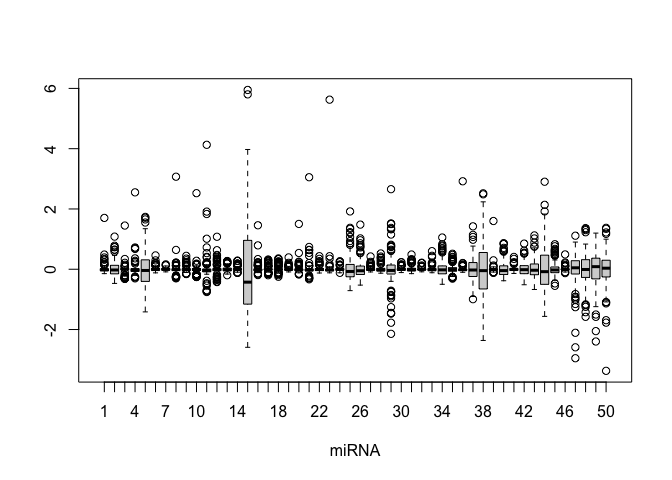
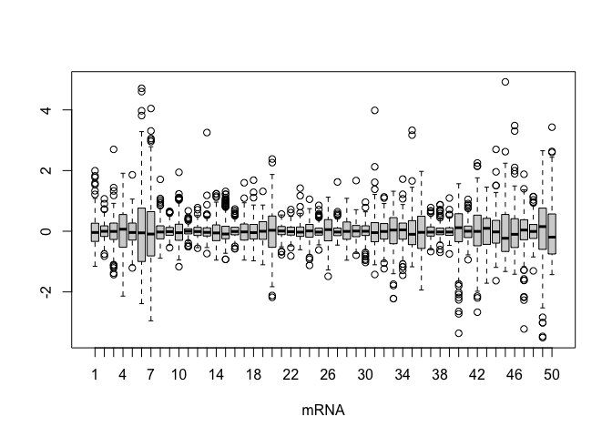
We consider some descriptive statistics, including the RV coefficient, a generalization of the Pearson correlation coefficient. We will not interpret them though.
# The range of the variances (note that data have mean zero)
cat("Range variances miRNA: \n")
## Range variances miRNA:
range(colSums(miRNA^2))
## [1] 0.2847355 808.2005360
cat("Range variances mRNA: \n")
## Range variances mRNA:
range(colSums(mRNA^2))
## [1] 2.875393 2603.933712
# Boxplots
boxplot(miRNA[,1:50], xlab="miRNA")
boxplot(mRNA[,1:50], xlab="mRNA")
## RV coefficient
# First define a function that calculates the trace of a matrix
tr <- function(X) sum(diag(X))
# Then calculate the RV coefficient
cat("RV coefficient between miRNA - mRNA: \n")
## RV coefficient between miRNA - mRNA:
tr(tcrossprod(miRNA)%*%tcrossprod(mRNA)) /
  sqrt(tr(crossprod(tcrossprod(miRNA)))*tr(crossprod(tcrossprod(mRNA))))
## [1] 0.4190371
Selecting the number of components
In the JIVE paper, the authors selected 5 joint, 13 miRNA-specific, and 33 mRNA-specific components. We will briefly look at the cross-validation and scree-plots to get an idea.
Cross-validation
We will first run cross-validation and scree-plots to get an idea of the latent structure. Note that the mRNA data contains 20k columns, which means that an O2PLS fit will take fairly long (try it, o2m(miRNA, mRNA, 5, 13, 33), it takes around 10 or 20 seconds). This will mean that a cross-validation takes much longer.
To cheat our way around this, we only consider the 20% of mRNA variables with the highest variance in the cross-validation. We further only look at varying numbers of joint components (yes, I know it’s very ad-hoc, but in a blog it’s allowed to cheat!). It seems that there are several minima (MSE around 1.35),and the smallest one is 8. So 5 joint components seems reasonable.
# Cross-validate with 25% of mRNA columns
mRNA_20 <- mRNA[,order(colSums(mRNA^2), decreasing = TRUE)[1:(0.20*ncol(mRNA))]]
crossval_o2m_adjR2(miRNA, mRNA_20, 3:15, 13, 33,
                   nr_folds = 2, nr_cores = detectCores())
## minimum is at n = 10
## Elapsed time: 57.29 sec
##         MSE  n nx ny
## 1  1.428345  3 13 33
## 2  1.417542  4 13 33
## 3  1.429473  5 13 33
## 4  1.403167  6 13 33
## 5  1.412174  7 13 33
## 6  1.409984  8 13 33
## 7  1.418884  9 13 33
## 8  1.399651 10 13 33
## 9  1.400566 11 13 33
## 10 1.413676 12 13 33
## 11 1.414905 13 13 33
## 12 1.411674 14 13 33
## 13 1.401464 15 13 33
Scree-plots
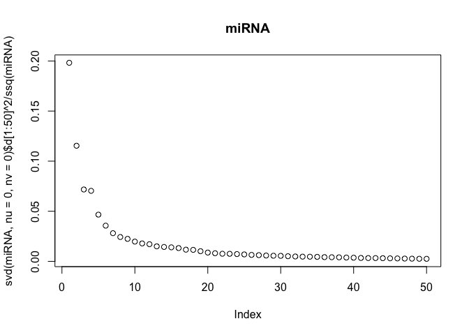
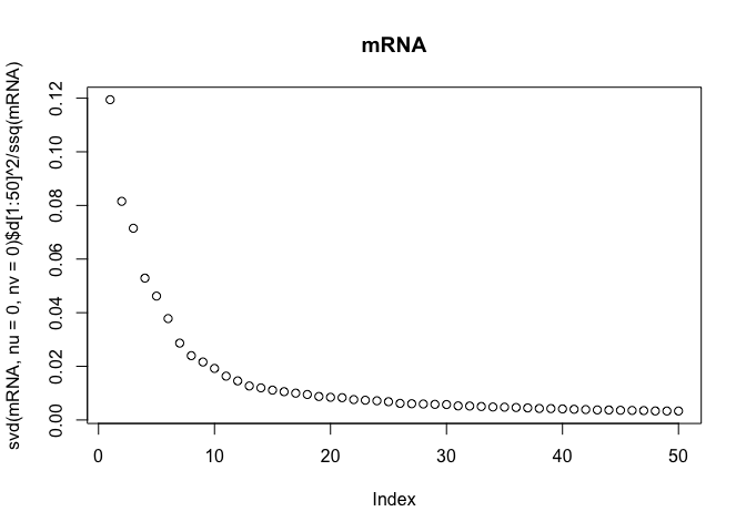
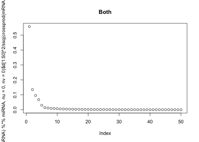
The scree-plots are much faster than cross-validation, and therefore an attractive alternative. Anyway, judging from the last plot where the eigenvalues of the covariance is shown, 4 joint components seem reasonable. Keeping in mind that 4 components are already selected, the other two scree-plots can be interpreted to get possible numbers of specific components.
Also, note that ssq(X) == sum(svd(X)$d^2) for any matrix X, where ssq(X) is defined as $\sum_{i,j} X_{ij}^2$. Check for yourself by computing the two quantities in R.
# plot the eigenvalues of the datasets
plot(svd(miRNA, nu=0, nv=0)$d[1:50]^2 / ssq(miRNA), main="miRNA")
plot(svd(mRNA, nu=0, nv=0)$d[1:50]^2 / ssq(mRNA), main="mRNA")
plot(svd(t(mRNA) %*% miRNA, nu=0, nv=0)$d[1:50]^2 / ssq(crossprod(mRNA, miRNA)),
     main="Both")
Fitting with OmicsPLS
As said before, we just take the numbers of components that were proposed in the JIVE article: 5 joint, 13 miRNA- and 33 mRNA-specific. Let’s fit!
fit <- o2m(miRNA, mRNA, 5, 13, 33)
fit
## O2PLS fit
## with 5 joint components
## and  13 orthogonal components in X
## and  33 orthogonal components in Y
## Elapsed time: 29.142 sec
summary(fit)
##
## *** Summary of the O2PLS fit ***
##
## -  Call: o2m(X = miRNA, Y = mRNA, n = 5, nx = 13, ny = 33)
##
## -  Modeled variation
## -- Total variation:
## in X: 34111.17
## in Y: 2108460
##
## -- Joint, Orthogonal and Noise as proportions:
##
##            data X data Y
## Joint       0.411  0.255
## Orthogonal  0.129  0.299
## Noise       0.460  0.446
##
## -- Predictable variation in Y-joint part by X-joint part:
## Variation in T*B_T relative to U: 0.772
## -- Predictable variation in X-joint part by Y-joint part:
## Variation in U*B_U relative to T: 0.662
##
## -- Variances per component:
##
##             Comp 1     Comp 2    Comp 3    Comp 4    Comp 5
## X joint   4670.569   2248.226  2199.626  2566.562  2347.516
## Y joint 214635.904 119396.667 97903.302 66598.520 39442.864
##
##          Comp 1  Comp 2  Comp 3  Comp 4  Comp 5  Comp 6  Comp 7  Comp 8  Comp 9
## X Orth 1066.899 533.912 457.206 431.636 319.001 339.482 286.003 271.197 222.029
##        Comp 10 Comp 11 Comp 12 Comp 13
## X Orth 227.613 215.702 213.275 181.551
##
##          Comp 1   Comp 2   Comp 3   Comp 4   Comp 5   Comp 6   Comp 7   Comp 8
## Y Orth 106501.5 57489.43 52113.68 51366.63 43339.43 40405.68 38746.07 23175.89
##          Comp 9  Comp 10  Comp 11  Comp 12  Comp 13  Comp 14  Comp 15  Comp 16
## Y Orth 23424.86 23283.06 18983.33 25658.53 15737.24 17717.82 14182.94 13418.37
##         Comp 17  Comp 18  Comp 19  Comp 20 Comp 21  Comp 22  Comp 23 Comp 24
## Y Orth 14754.61 11547.62 11799.25 11896.08 11319.9 9940.961 10286.65 10190.8
##         Comp 25  Comp 26  Comp 27  Comp 28  Comp 29  Comp 30  Comp 31  Comp 32
## Y Orth 8912.932 8484.911 8400.586 8658.311 8298.798 7751.376 7271.087 7431.346
##         Comp 33
## Y Orth 7336.554
##
##
## -  Coefficient in 'U = T B_T + H_U' model:
## -- Diagonal elements of B_T =
##  6.733 6.315 6.95 4.135 3.599
So apparently, O2PLS has captures 41% of the miRNA variation and 26% of the mRNA variation as joint variation. Also, 13% resp. 30% was specific variation. Note that around 77%*26%=20% of the variation in mRNA is predictable with miRNA. One can check the literature (or the experts) if these numbers make sense.
A plot of the scores
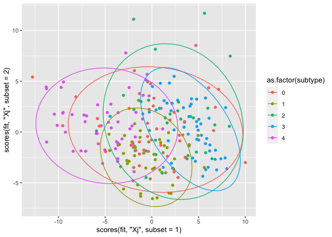
We finally arrived at the scores plot. This plot shows the scores of each sample, and when colored according to their subtype, differentiation might be spotted. For this plot, we use ggplot and add 95% confidence ellipses. Note that the scores function can be used, but a basic subsetting of the relevant scores object Tt or U is also fine.
Here are the subtype definitions from the Readme.txt:
0: Unclassified 1: Classical 2: Neural 3: Proneural 4: Mesanchymal
qplot(x = scores(fit, "Xj",subset = 1),
      y = scores(fit, "Xj", subset = 2),
      col = as.factor(subtype)) + stat_ellipse()
qplot(x=fit$U[,1], y=fit$U[,2], col = as.factor(subtype)) + stat_ellipse()
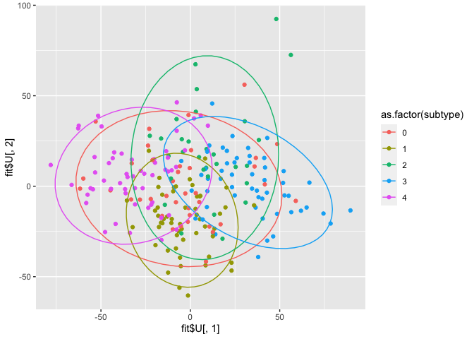
There is some differentiation between subtype 3 and 4 in component 1. Subtype 1 is quite homogeneous, and especially present in component 2. These results are similar for miRNA as well as mRNA, though the latter seems to yield more distinct groups.
Since we don’t have the gene IDs for the columns, it’s impossible to do further gene enrichment analysis. However, the scores plot is already quite similar to JIVE’s output.
Conclusions
OmicsPLS can be used to analyse transcriptomics and miRNA-omics data from cancer patients. We redid the analysis in the JIVE article and showed the results. The cross-validation and scree plots seemed to agree somewhat with the numbers of components that were proposed in JIVE. The final scores plot colored according to the cancer subtypes was similar to the plot in the original article.